Lab 6

Statistical tests

Overview

While I encourage you to run any test of your choosing, you’ll likely end up using FIsher’s exact/chi-squared test.

Chi-squares: https://www.westga.edu/academics/research/vrc/assets/docs/ChiSquareTest_LectureNotes.pdf /
T-test: https://toltex.imag.fr/TwoTestSPLS/
Fisher’s exact: https://www.biostat.jhsph.edu/~iruczins/teaching/140.652/supp21.pdf /

We will also practice material learned so far to reinforce some of the code learned so far. This week, we’ll learn how to perform chi-square tests. To do so, I am using Mike Love and Irizarry’s book (recommended for life sciences). You can also visit Mike Love’s github page to use the book online here.

Loading libraries

library(tidyverse)
library(ggplot2)

Loading the file: You need not worry about this chunk. You may simply run it. Or you could also download the mice dataset from the website and read in as a csv file for practice.

dir <- "https://raw.githubusercontent.com/genomicsclass/dagdata/master/inst/extdata/"
url <- paste0(dir, "femaleMiceWeights.csv")
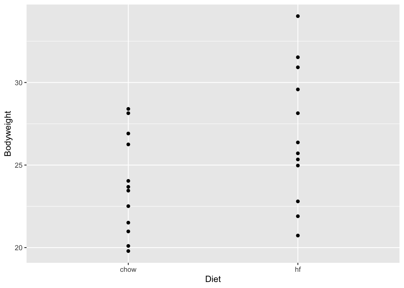
dat <- read.csv(url)

Student exercise 1. How many mice are in this dataset? 2. Calculate mean weight of the mice 3. Create a scatter plot (like the one I’ve already created) 4. What is the difference in mean weight by diet of the mice?

  mean_wt_hf
1   3.020833

Performing chi-squares and t-tests.

Let’s understand the syntax for both these tests and use p-values to determine significance.

# Perform a t-test for one categorical and one continuous var
t.test(Bodyweight ~ Diet, data = dat)


    Welch Two Sample t-test

data:  Bodyweight by Diet
t = -2.0552, df = 20.236, p-value = 0.053
alternative hypothesis: true difference in means between group chow and group hf is not equal to 0
95 percent confidence interval:
 -6.08463229  0.04296563
sample estimates:
mean in group chow   mean in group hf 
          23.81333           26.83417

# Chi-square requires at least 30 observations, so not ideal in this case
# Also, we do not have two categorical vars so we could recode the weight as high vs low
print(mean(dat$Bodyweight))

[1] 25.32375

dat_new <- 
  dat %>% 
  mutate(new_weight = if_else(Bodyweight > 25.32375, 'High', 'Low'))

test <- chisq.test(table(dat_new$Diet, dat_new$new_weight))
test


    Pearson's Chi-squared test with Yates' continuity correction

data:  table(dat_new$Diet, dat_new$new_weight)
X-squared = 1.5, df = 1, p-value = 0.2207

# Fisher's exact

fisher.test(dat_new$Diet, dat_new$new_weight)


    Fisher's Exact Test for Count Data

data:  dat_new$Diet and dat_new$new_weight
p-value = 0.2203
alternative hypothesis: true odds ratio is not equal to 1
95 percent confidence interval:
 0.03289187 1.77138188
sample estimates:
odds ratio 
 0.2661096

To Do

Nothing!!! This marks the end of our lab section - let’s spend time practicing.